Validation criteria

(Note that in order to answer some of the questions on this page, you must be able to access the coordinates of some PDB entries. You can find links to the three major wwPDB sites (from which you can retrieve coordinates) on the page with Useful links. And instead of a graphics program that runs on your machine you may also want to use one of the interactive visualisation methods offered by the various wwPDB sites.)

Refresher:

• If you have forgotten what amino acids are, look here or here (alternative)
• If you have forgotten what molecular geometry is, look here (alternative)
• If you have forgotten what dihedral or torsion angles are, look here (alternative)
• If you have forgotten what eclipsed and staggered conformations are, look here (alternative)
• If you have forgotten what chiral carbon atoms are, look here
• If you have forgotten what phi and psi are, look here or here
• If you have forgotten what chi-1, chi-2 etc. are, look here

Coordinates and temperature factors

• The covalent geometry of a model can be assessed by comparing bond lengths and angles to a library of "ideal" values. In the past, every refinement and modelling program had its own set of "ideal" values. This even made it possible to detect (with 95% accuracy) with which program a model had been refined, simply by inspecting its covalent geometry. Nowadays, standard sets of ideal bond lengths and bond angles, derived from an analysis of small-molecule crystal structures, are available for proteins and nucleic acids.

  For bond lengths, the RMS deviation from ideal values is invariably quoted. Deviations from ideality of bond angles can be expressed directly as an angular RMS deviation or in terms of angle distances (i.e., the angle ABC is measured by the 1-3 distance |AC|).

  Other checks in this class include chirality and planarity tests.

  Validation potential of geometric tests: poor. Good scores for these criteria prove little. However, if an entire model scores poorly, this should set off warning bells. Also, gross outliers should always be investigated!

  Q. 2. Which amino acids contain chiral carbon atoms? Are there any amino acids that contain more than one chiral carbon atom? If so, which one(s)? (If you have forgotten what the side chains of the 20 common amino acids look like, check here, here, here, or here.)

  Q. 3. PDB entry 5RXN contains three threonine residues, named 5, 7 and 28. Inspect these three residues with your favourite graphics program. Does anything strike you as odd?

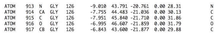
  Q. 4. Look up Gly 126 in the PDB file (i.e., not the structure) of entry 1VNS. Before the PDB remediation in 2007, this residue looked as follows: What differences do you notice?

  Q. 5. Do you expect the CB of a tyrosine residue to lie in the same plane as the aromatic ring?

  Q. 6. Using your favourite graphics program, have a look at residue TRP D67 in PDB entry 7GPB. Does anything strike you as odd?

  Q. 7. Using your favourite graphics program, compare aspartates C168 and C169 in PDB entry 1DLP. Does anything strike you as odd?

• The conformation of the backbone of every non-terminal amino acid residue is determined by three torsion angles, traditionally called:
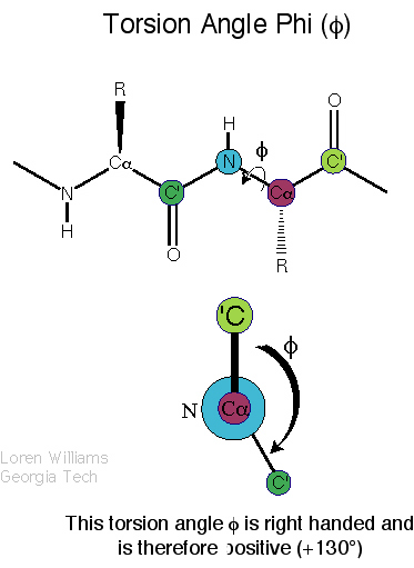
  • phi (C[i-1]-N[i]-CA[i]-C[i])
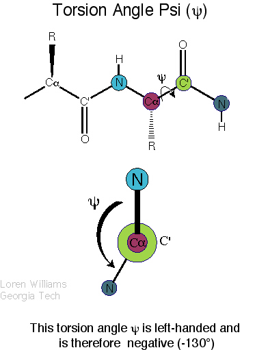
  • psi (N[i]-CA[i]-C[i]-N[i+1])
  • omega (CA[i]-C[i]-N[i+1]-CA[i+1])
  Due to resonance, the peptide bond has partial double-bond character. Therefore, the omega angle is restrained to values near 0 (cis-peptide) and 180 degrees (trans-peptide). Cis-peptides are relatively rare and usually (but not always) occur if the next residue is a proline. The omega angle therefore offers little in the way of validation checks, although values in the range of ±20 to ±160 degrees should be treated with caution in anything but very high-resolution models.

  Validation potential of omega: poor.

  Resonance forms of a typical peptide group. The uncharged, single-bonded form (typically ~60%) is shown on the left, whereas the charged, double-bonded form (typically ~40%) is on the right. (Image and caption reproduced from Wikipedia.)

  The phi and psi torsion angles, on the other hand, are much less restricted, but it has been known for a long time that, due to steric hindrance, there are several clearly preferred combinations of phi, psi values (a scatter plot of phi,psi values for all residues in a protein model is called a Ramachandran plot). This is true even for proline and glycine residues, although their distributions are atypical. Also, an overwhelming majority of residues that are not in regular secondary structure elements are found to have favourable phi, psi torsion-angle combinations. For these reasons, the Ramachandran plot is an extremely simple, useful and sensitive indicator of model quality. Residues that have unusual phi, psi torsion-angle combinations should be scrutinised by the crystallographer. If they have convincing electron density, there is probably a good structural or functional reason for the protein to tolerate the energetic strain that is associated with the unusual conformation. The quality of a model's Ramachandran plot is most convincingly illustrated with a figure. Alternatively, the fraction of residues in certain predefined areas of the plot (e.g., core regions) can be quoted, but in that case it is important to indicate which definition of such areas was used.

  If you are interested in finding out which specific steric clashes put restrictions on phi and/or psi, read the 2003 paper by Ho et al. They find that O(i-1)...CB(i) restricts phi of residue i, CB(i)...O(i) and CB(i)...N(i+1) restrict psi, and O(i-1)...O(i) and O(i-1)...N(i+1) restrict both phi and psi.

  Validation potential of phi, psi combinations: excellent. A quick look at the Ramachandran plot will tell you a lot about the quality of a model. Good models have most residues tightly clustered in the most-favoured regions with relatively few outliers. Good, but low-resolution models may have less pronounced clustering, but will still have few outliers. Models that show poor clustering and many outliers are bound to be poor.

  Definition of phi?	Definition of psi?

  Q. 8a. The two images above show the definition of the phi and psi torsion angles. However, one of the figures contains a mistake. What is the mistake? Does it matter?

  Rotation around phi	Rotation around psi
  The animations above show how steric clashes (pink dashed lines) develop during rotation around phi and psi, respectively. (If the animation has stopped, click the Refresh or Reload button in your browser while holding down the SHIFT key.) Can you identify all the atoms that are shown? Hint: hydrogen atoms are white. (Images kindly provided by David Sanders, University of Saskatchewan.)

  Q. 8b. What is the value of psi in the animation on the left? And what is the value of phi in the animation on the right? Explain why (phi, psi) combinations near (0, 0) are forbidden for all residue types.

  Distribution of phi, psi angle combinations for more than 80,000 residues. Densely populated regions are shown in blue and green, whereas red and orange indicate scarcely populated areas. Similar figures for each of the twenty amino-acid residue types can be found here.

  Q. 9. The three most-densely populated areas in the Ramachandran plot are called the alpha, the beta, and the left-handed helical region. Where are these three regions located approximately in the Ramachandran plot?

  Q. 10. Why do glycine residues have an atypical distribution? And proline residues?

  Q. 11. In general, positive phi values are much less favourable than negative ones. Can you explain why this is so? (Hint: the phi rotation animation may be of help. Positive phi values occur when the previous residue's carbonyl oxygen atom points into the screen.) Is it also true for glycine residues? And how about D-amino acids?

  Q. 12. Which regions would you expect to be most favourable in the Ramachandran plot of a protein that consists entirely of D-amino acids?

  Q. 13. For the PDB entry 3LZ2 a Ramachandran plot is available calculated with four different programs: WHAT IF PROCHECK MOLEMAN2 MolProbity Do these programs have the same "opinion" about the quality of the Ramachandran plot of this model? What does this teach you?

• All amino-acid residues whose side chain extends beyond the CB atom have one or more conformational side-chain torsion angles, termed chi-1 (N-CA-CB-XG; where X may be carbon, sulfur, or oxygen, depending on the residue type; if there are two G atoms, the chi-1 torsion is calculated with reference to the atom with the lowest numerical identifier, e.g., OG1 for threonine residues), chi-2 (CA-CB-XG-XD), etc.

  Validation potential of chi torsions: moderate.

  Distribution of chi-1 angle values for more than 67,000 residues. Similar figures for chi-2 to chi-4 can be found here.

  Q. 14. What are the three conformations that give rise to local maxima in the chi-1 distribution called?

  Q. 15. Can you explain why there appear two "humps" in the chi-1 distribution near +35 and -35 degrees?

  Early on, it was found that the values that these torsion angles assume in proteins are similar to those expected on the basis of simple energy calculations and that, in addition, certain combinations of chi-1, chi-2 values are clearly preferred (so-called [preferred] rotamer conformations). Analogous to Ramachandran plots, chi-1, chi-2 scatter plots can be produced that show how well a protein's side-chain conformations conform to known preferences. Alternatively, for each residue, a score can be computed that shows how similar its side-chain conformation is to that of the most similar rotamer for that residue type. This score can be calculated as an RMS distance between corresponding side-chain atoms, or it can be expressed as an RMS deviation of side-chain torsion-angle values from those of the most similar rotamer.

  Validation potential of chi combinations: excellent.

  Distribution of chi-1 (horizontal), chi-2 (vertical) angle combinations for more than 47,000 residues. Densely populated regions are shown with contours. Similar figures for individual amino-acid residue types can be found here.

  Q. 16. How many clear rotamer conformations exist for leucine residues?

  Q. 17. In the plot of the chi-2 distribution, where do you expect to find most of the proline residues? What are the two most favourable rotamers that you expect to find for proline?

  Q. 18. Asp, Asn and His have similar chi-1, chi-2 distributions. What is strange about these distributions? Can you explain this? Why don't Gln and Glu suffer from this? (Plots of the distributions can be found here.)

• In the past (and sometimes still today ...), "hot" or preliminary models were sometimes deposited as a "CA-only model" (i.e., only the coordinates of the CA atoms were deposited). However, not many validation tools can handle such models. The CA backbone can be characterised by CA-CA distances (~2.9 Å for a cis-peptide, and ~3.8 Å for a trans-peptide), CA-CA-CA pseudo-angles, and CA-CA-CA-CA pseudo-torsion angles. The pseudo-angles and torsion angles turn out to assume certain preferred value combinations, much like the backbone phi and psi torsions, and this can be employed for the validation of CA-only models.

  Validation potential of CA-only tests: good. But they provide little in the way of error diagnostics.

  Distribution of CA-CA-CA pseudo-angles (horizontal) and CA-CA-CA-CA pseudo-torsions (vertical) for a large number of high-resolution structures. More information can be found here.

  Example of a "CA-Ramachandran plot" for a high-resolution model.

• Hydrophobic, electrostatic, and hydrogen-bonding interactions are the main stabilising forces of protein structure. This leads to packing arrangements where hydrophobic residues tend to interact with each other, where charged residues tend to be involved in salt links, and where hydrophilic residues prefer to interact with each other or to point out into the bulk solvent. Serious model errors will often lead to violations of such simple rules of thumb and introduce non-physical interactions (e.g., a charged arginine residue located inside a hydrophobic pocket) that serve as good indicators of model errors. Directional atomic contact analysis (DACA) is a method in which these empirical notions have been formalised through database analysis. For every group of atoms in a protein, it yields a score which, in essence, expresses how "comfortable" that group is in its environment in the model under scrutiny (compared to the expectations derived from the database). If a region in a model (or the entire model) has consistently low scores, this is a very strong indication of model errors.

  Validation potential of DACA analysis: excellent.

• Sometimes a protein crystallises with more than one independent copy whose structure needs to be determined separately - this phenomenon is called non-crystallographic symmetry (NCS). Since all copies have the same sequence and chemical composition, we expect that the models of the various independent copies should be very similar. During model refinement, a careful crystallographer might either constrain the various copies to be identical, or restrain them to be very similar in terms of their structure. This reduces the effective number of parameters (degrees-of-freedom) in the model and tends to result in better determined models. Large, random differences in models related by NCS are often indicative of poor refinement practices, and sometimes result in poor models. Hence, the similarity of the NCS-related models can be used as a validation criterion. This similarity can be expressed in terms of RMS distances between equivalent atoms in the two (or more) copies of the molecule. Alternatively, differences between corresponding phi, psi and chi torsion angles can be used.

  Validation potential of NCS checks: moderate. NCS constraints and restraints are so powerful that it is usually better to impose them during refinement (especially at low resolution) than to use NCS as an a posteriori validation criterion.

• In crystallographic refinement, Atomic Displacement Parameters (ADPs; often referred to as temperature factors or B-factors) model the effects of thermal vibration of the atoms. Except at high resolution (typically, better than ~1.5 Å) where there are sufficient observations to warrant refinement of anisotropic temperature factors, ADPs are usually constrained to be isotropic. The isotropic temperature factor B of an atom is related to the atom's mean-square displacement. Compared to the atomic coordinates, there are usually few restraints on temperature factors during refinement. Therefore, particularly at low resolution, temperature factors often function as "error sinks". They absorb not only the effects of thermal vibration but also of static and dynamic disorder and of various kinds of model errors.

  Compared to the wealth of statistics that can be used to check and validate coordinates, there are relatively few methods available to assess how reasonable a model's temperature factors are. One should keep in mind that a low average B-factor, per se, is not necessarily an indication of high model quality. For instance, a backwards-traced protein model can have a considerably lower average B-factor than a correct model at a similar resolution. Average (and minimum and maximum) temperature-factor values are sometimes listed separately for various groups of atoms (e.g., individual protein or nucleic acid molecules, ligands, solvent molecules). A simple plot of residue-averaged temperature factors as a function of residue number may reveal regions of the molecule that have consistently high B-factors, which may be due to problems in the model.

  Other statistics pertain to the RMS differences in B-factors between atoms that are somehow related, for example through a chemical bond or by NCS. Sometimes these statistics are calculated separately for main-chain and side-chain atoms. If the B-factors of such related atoms have been restrained to be similar during refinement, these checks do not provide a convincing indication of the quality of the model.

  Given experimental data (preferably to better than 3 Å resolution) and some knowledge of the contents of the unit cell, an overall temperature factor can be calculated that is known as the Wilson B-factor. In practice (see figure below), there is a good correlation between the model and the Wilson B factors, so very large discrepancies between them could suggest that the B-factors of the model need to be taken with a grain of salt.

  Validation potential of temperature-factor tests: poor.

  Correlation between average model B-factor and Wilson B-factor, including data for >21,000 EDS entries. (If you don't know how to interpret this type of box plot, look here.)

Model versus experimental data

• One of the major determinants of the quality of the model ought to be the resolution of the experimental data that was used to determine it. Higher resolution means more experimental data, and more detailed information contained in that data. The nominal resolution limits of a dataset are chosen by the crystallographer. Unfortunately, due to the subjective nature of this process, resolution limits cannot be compared meaningfully between datasets processed by different crystallographers. One day, hopefully, the term "resolution" will be replaced by an estimate of the information content of the data. Nevertheless, in most cases one would a priori expect a model to be more reliable if it is advertised as a 1.5 Å model, than if it is based on 3 Å data.

  Validation potential of resolution: moderate.

• The major source of crystallographic data used in model refinement is the set of so-called "observed structure-factor amplitudes" (|F_obs|, derived from the observed reflection intensities). From the model alone, calculated structure-factor amplitudes can be derived (|F_calc|). The traditional statistic used to assess how well a model fits the experimental data is the crystallographic R-value:

      R = { SUM weight * | |Fobs| - scale * |Fcalc| | } / { SUM weight * |Fobs| }
      

  This statistic is closely related to the standard least-squares crystallographic residual:

      SUM weight * ( |Fobs| - scale * |Fcalc| )2
      

  and its value can be reduced essentially arbitrarily by increasing the number of parameters used to describe the model or, conversely, by reducing the number of experimental observations or the number of restraints imposed on the model. Therefore, the conventional R-value is only meaningful if the number of experimental observations and restraints greatly exceeds the number of model parameters.

  Validation potential of R: poor. Only at very high resolution does the conventional R-value become well-determined and, hence, reliable and informative.

  In 1992, Brünger introduced the free R-value (R_free), whose definition is identical to that of the conventional R-value, except that the free R-value is calculated for a small subset of reflections that is not used in the refinement of the model. The free R-value therefore measures how well the model predicts experimental observations that are not used to fit the model (cross-validation).

  Until the mid-1990s, a conventional R-value below 0.25 was generally considered to be a sign that a model was essentially correct. While this is probably true at high resolution, it was subsequently shown for several intentionally mistraced models that these can be refined to deceptively low conventional R-values. Brünger suggests a threshold value of 0.40 for the free R-value, i.e., models with free R-values greater than 0.40 should be treated with caution. Since the difference between the conventional and free R-value is partly a measure of the extent to which the model over-fits the data (i.e., some aspects of the model improve the conventional but not the free R-value and are therefore likely to fit noise rather than signal in the data), this difference R_free - R should be small (ideally < 0.05).

  If you want to see some plots of the relation between R, R_free, R_free - R and resolution (for structures deposited from 1991 to 2000), look here.

  Validation potential of R_free: excellent. Gives a quick indication about the overall quality of the model.

  Validation potential of R_free - R: good. Gives a quick indication of the extent to which the experimental data has been over-fitted. However, if a model is very incomplete it may also display a high value for this quantity.

• The fit of a model to the data can also be assessed more directly and locally for specific groups of atoms. Jones et al. introduced the real-space R-value, which measures the similarity of an electron-density map calculated directly from the model (rho_calc) and one that incorporates experimental data (rho_obs) as:

      RSR = SUM | rhoobs - rhocalc | / SUM | rhoobs + rhocalc |
      

  where the sums extend over all grid points in the map that surround the selected set of atoms (e.g., one residue). The real-space fit can also be expressed as a correlation coefficient (RSCC), which has the advantage that no scaling of the two densities is necessary.

  Validation potential of RSR and RSCC: good. (Provided the experimental map is not biased too much by the model.)

• Since a measurement without an error estimate is not a measurement, crystallographers are keen to assess the estimated errors in the atomic coordinates and, by extension, in the atomic positions, bond lengths, etc. In principle, upon convergence of a least-squares refinement, the variances and covariances of the model parameters can be calculated, but this requires enormous computational resources. Therefore, one of a battery of (sometimes quasi-empirical) approximations is usually employed. These include Luzzati plots (cross-validated or not), "SIGMAA" plots (cross-validated or not) and the DPI (Diffraction-only Precision Indicator). The cross-validated methods appear to give reasonable error estimates.

  Validation potential of coordinate estimates: moderate if cross-validated, otherwise poor.

Latest update on 26 January, 2009.